Introduction to Neural Networks with PyTorch

ICCS Summer School 2024

Matt Archer

ICCS/Cambridge

Surbhi Goel

ICCS/Cambridge

Rough Schedule

9:00-9:30 - NN lecture
9:30-10:30 - Teaching/Code-along
10:30-11:00 - Coffee
11:00-12:00 - Teaching/Code-along

Lunch

12:00 - 13:30

Helping Today:

Person 1 - Cambridge RSE

Material

These slides can be viewed at:

https://cambridge-iccs.github.io/practical-ml-with-pytorch

The html and source can be found on GitHub. Follow this link:

https://tinyurl.com/ml-iccs-24

Based on the workshop developed by Jack Atkinson and Jim Denholm:

V1.0 released and JOSE paper accepted:

(Atkinson and Denholm 2024)

Part 1: Neural-network basics – and fun applications.

Stochastic gradient descent (SGD)

Generally speaking, most neural networks are fit/trained using SGD (or some variant of it).
To understand how one might fit a function with SGD, let’s start with a straight line: \[y=mx+c\]

Fitting a straight line with SGD I

Question—when we a differentiate a function, what do we get?

Consider:

\[y = mx + c\]

\[\frac{dy}{dx} = m\]

\(m\) is certainly \(y\)’s slope, but is there a (perhaps) more fundamental way to view a derivative?

Fitting a straight line with SGD II

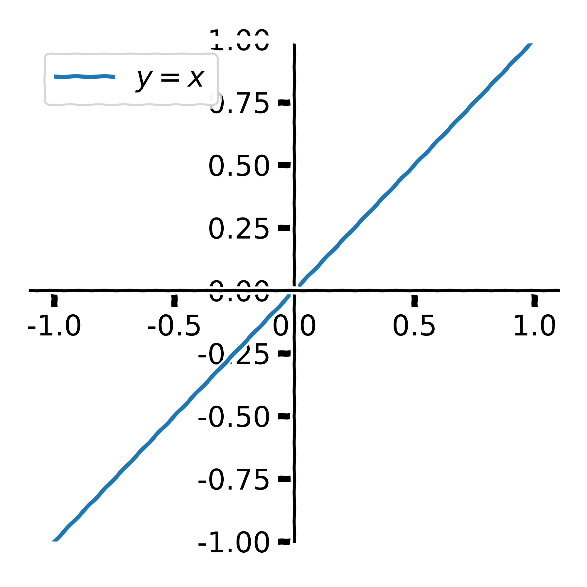
Answer—a function’s derivative gives a vector which points in the direction of steepest ascent.

Consider

\[y = x\]

\[\frac{dy}{dx} = 1\]

What is the direction of steepest descent?

\[-\frac{dy}{dx}\]

Fitting a straight line with SGD III

When fitting a function, we are essentially creating a model, \(f\), which describes some data, \(y\).
We therefore need a way of measuring how well a model’s predictions match our observations.

Consider the data:

\(x_{i}\)	\(y_{i}\)
1.0	2.1
2.0	3.9
3.0	6.2

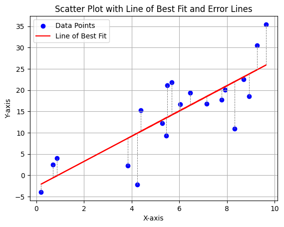
We can measure the distance between \(f(x_{i})\) and \(y_{i}\).
Normally we might consider the mean-squared error:

\[L_{\text{MSE}} = \frac{1}{n}\sum_{i=1}^{n}\left(y_{i} - f(x_{i})\right)^{2}\]

We can differentiate the loss function w.r.t. to each parameter in the the model \(f\).
We can use these directions of steepest descent to iteratively ‘nudge’ the parameters in a direction which will reduce the loss.

Fitting a straight line with SGD IV

Model: \(f(x) = mx + c\)
Data: \(\{x_{i}, y_{i}\}\)
Loss: \(\frac{1}{n}\sum_{i=1}^{n}(y_{i} - x_{i})^{2}\)

\[ \begin{align} L_{\text{MSE}} &= \frac{1}{n}\sum_{i=1}^{n}(y_{i} - f(x_{i}))^{2}\\ &= \frac{1}{n}\sum_{i=1}^{n}(y_{i} - mx_{i} + c)^{2} \end{align} \]

We can iteratively minimise the loss by stepping the model’s parameters in the direction of steepest descent:

\[m_{n + 1} = m_{n} - \frac{dL}{dm} \cdot l_{r}\]

\[c_{n + 1} = c_{n} - \frac{dL}{dc} \cdot l_{r}\]

where \(l_{\text{r}}\) is a small constant known as the learning rate.

Quick recap

To fit a model we need:

Some¹ data.
A model.
A loss function
An optimisation procedure (often SGD and other flavours of SGD).

What about neural networks?

Neural networks are just functions.
We can “train”, or “fit”, them as we would any other function:
- by iteratively nudging parameters to minimise a loss.
With neural networks, differentiating the loss function is a bit more complicated
- but ultimately it’s just the chain rule.
We won’t go through any more maths on the matter—learning resources on the topic are in no short supply.¹

Fully-connected neural networks

The simplest neural networks commonly used are generally called fully-connected neural nets, dense networks, multi-layer perceptrons, or artifical neural networks (ANNs).

We map between the features at consecutive layers through matrix multiplication and the application of some non-linear activation function.

\[a_{l+1} = \sigma \left( W_{l}a_{l} + b_{l} \right)\]

For common choices of activation function, see the PyTorch docs.

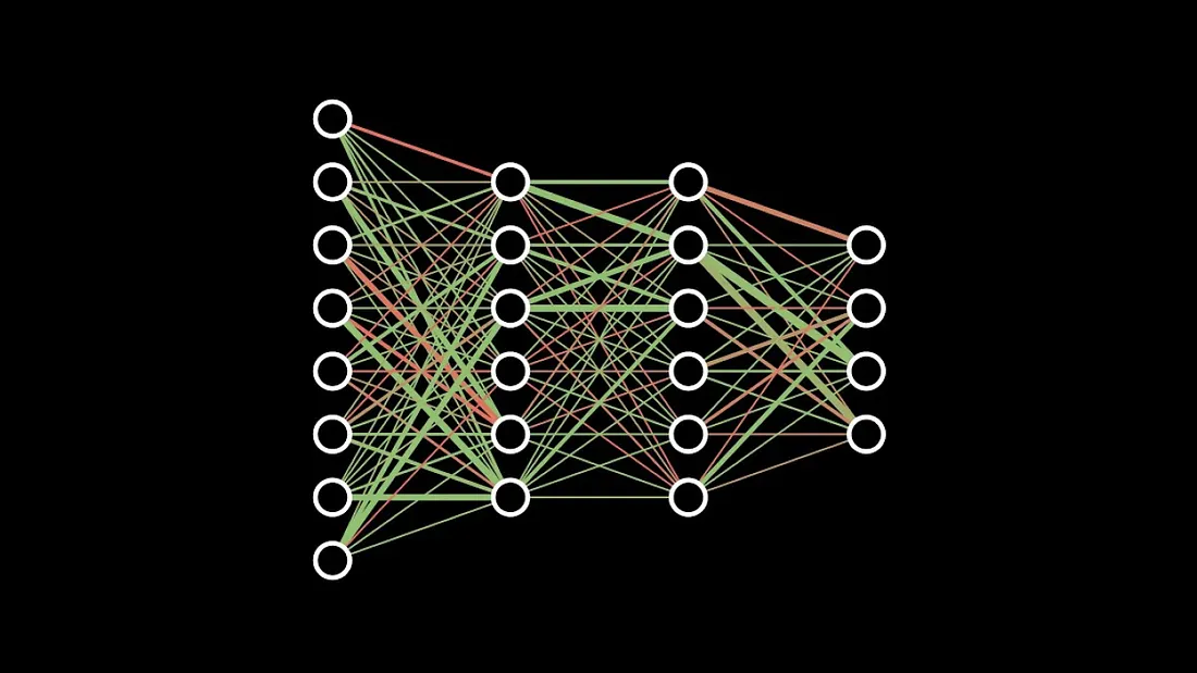
Image source: 3Blue1Brown

Uses: Classification and Regression

Fully-connected neural networks are often applied to tabular data.
- i.e. where it makes sense to express the data in a table-like object (such as a pandas data frame).
- The input features and targets are represented as vectors.

Neural networks are normally used for one of two things:
- Classification: assigning a semantic label to something – i.e. is this a dog or cat?
- Regression: Estimating a continuous quantity – e.g. mass or volume – based on other information.

Python and PyTorch

In this workshop, we will implement some straightforward neural networks in PyTorch, and use them for different classification and regression problems.
PyTorch is a deep learning framework that can be used in both Python and C++.
- I have never met anyone actually training models in C++; I find it a bit weird.
See the PyTorch website: https://pytorch.org/

Exercises

Penguins!

Image source: Palmer Penguins by Alison Horst

Exercise 1 – classification

In this exercise, you will train a fully-connected neural network to classify the species of penguins based on certain physical features.
https://github.com/allisonhorst/palmerpenguins

Exercise 2 – regression

In this exercise, you will train a fully-connected neural network to predict the mass of penguins based on other physical features.
https://github.com/allisonhorst/palmerpenguins

Part 2: Fun with CNNs

Convolutional neural networks (CNNs): why?

Advantages over simple ANNs:

They require far fewer parameters per layer.
- The forward pass of a conv layer involves running a filter of fixed size over the inputs.
- The number of parameters per layer does not depend on the input size.
They are a much more natural choice of function for image-like data:

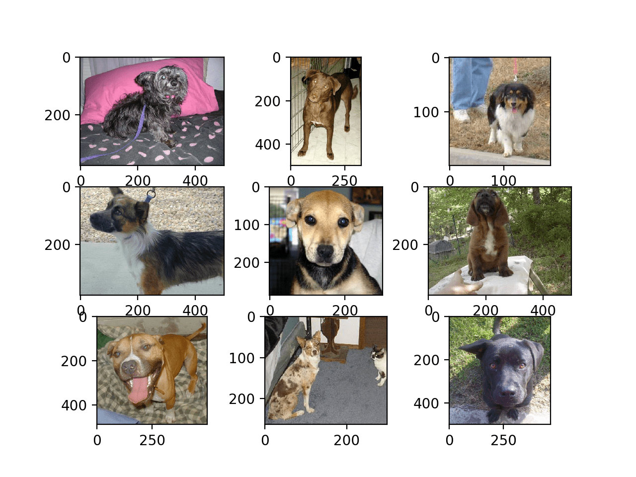
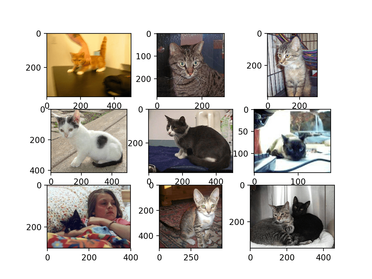
Image source: Machine Learning Mastery

Convolutional neural networks (CNNs): why?

Some other points:

Convolutional layers are translationally invariant:
- i.e. they don’t care where the “dog” is in the image.
Convolutional layers are not rotationally invariant.
- e.g. a model trained to detect correctly-oriented human faces will likely fail on upside-down images
- We can address this with data augmentation (explored in exercises).

What is a (1D) convolutional layer?

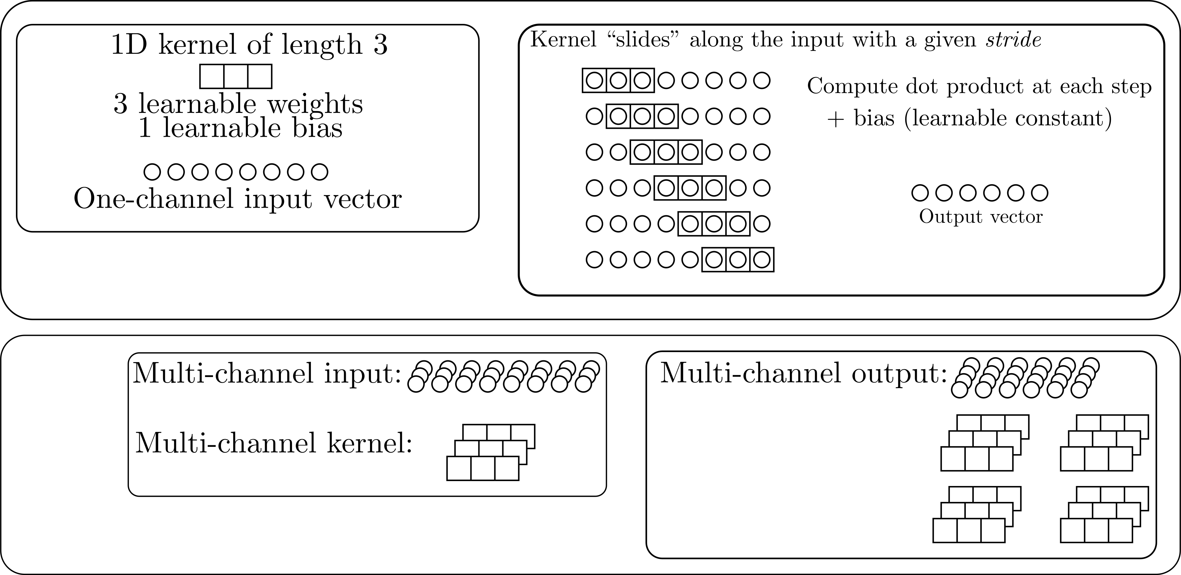
See the torch.nn.Conv1d docs

2D convolutional layer

Same idea as in on dimension, but in two (funnily enough).

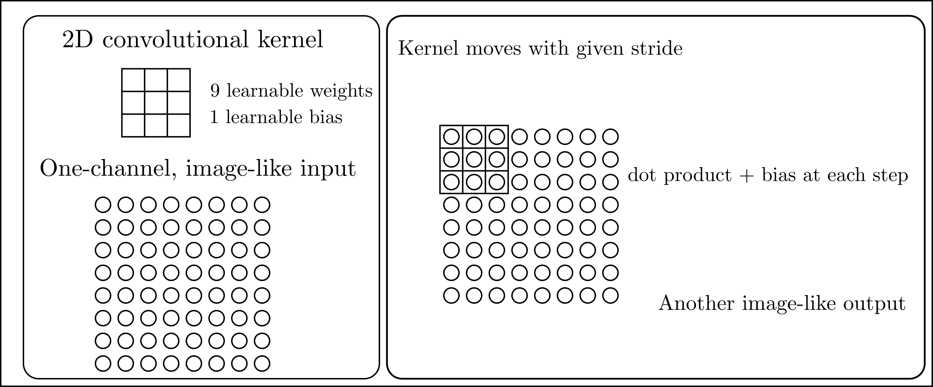
Everthing else proceeds in the same way as with the 1D case.
See the torch.nn.Conv2d docs.
As with Linear layers, Conv2d layers also have non-linear activations applied to them.

Typical CNN overview

Series of conv layers extract features from the inputs.
- Often called an encoder.
Adaptive pooling layer:
- Image-like objects \(\to\) vectors.
- Standardises size.
- torch.nn.AdaptiveAvgPool2d
- torch.nn.AdaptiveMaxPool2d
Classification (or regression) head.

For common CNN architectures see torchvision.models docs.

Image source: medium.com - binary image classifier cnn using tensorflow

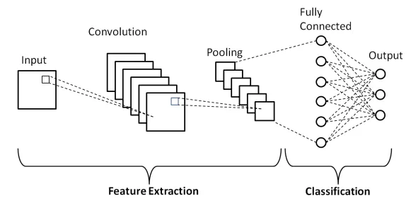
Exercises

Exercise 1 – classification

MNIST hand-written digits.

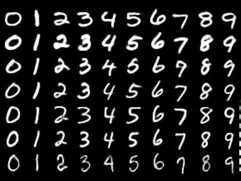
In this exercise we’ll train a CNN to classify hand-written digits in the MNIST dataset.
See the MNIST database wiki for more details.

Image source: npmjs.com

Exercise 2—regression

Random ellipse problem

In this exercise, we’ll train a CNN to estimate the centre \((x_{\text{c}}, y_{\text{c}})\) and the \(x\) and \(y\) radii of an ellipse defined by \[ \frac{(x - x_{\text{c}})^{2}}{r_{x}^{2}} + \frac{(y - y_{\text{c}})^{2}}{r_{y}^{2}} = 1 \]
The ellipse, and its background, will have random colours chosen uniformly on \(\left[0,\ 255\right]^{3}\).
In short, the model must learn to estimate \(x_{\text{c}}\), \(y_{\text{c}}\), \(r_{x}\) and \(r_{y}\).

Contact

For more information we can be reached at:

Matt Archer

Surbhi Goel

Jack Atkinson

@jatkinson1000@fosstodon.org

Jim Denholm

UoCambridge

jd949[AT]cam.ac.uk

jdenholm

You can also contact the ICCS, make a resource allocation request, or visit us at the Summer School RSE Helpdesk.

Atkinson, Jack, and Jim Denholm. 2024. “Practical machine learning with PyTorch.” Journal of Open Source Education 7 (76): 239. https://doi.org/10.21105/jose.00239.